Quickstart Guide
Basic Example
Import the HeartPy module and load a file
import heartpy as hp

hrdata = hp.get_data('data.csv')
This returns a numpy.ndarray.
Analysis requires the sampling rate for your data. If you know this a priori, supply it when calling the process() function, which returns a dict{} object containing all measures:
import heartpy as hp

#load example data
data, _ = hp.load_exampledata(0) #this example set is sampled at 100Hz

    working_data, measures = hp.process(data, 100.0)
process(dataset, sample_rate, windowsize=0.75, report_time=False, calc_freq=False, freq_method=’welch’, interp_clipping=False, clipping_scale=False, interp_threshold=1020, hampel_correct=False, bpmmin=40, bpmmax=180, reject_segmentwise=False, high_precision=False, high_precision_fs=1000.0, measures = {}, working_data = {})
requires two arguments:
- dataset: An 1-dimensional list, numpy array or array-like object containing the heart rate data;
- sample_rate: The samplerate of the signal in Hz;
Several optional arguments are available:
- windowsize: _optional_ windowsize is the window size used for the calculation of the moving average. The windowsize is defined as windowsize * samplerate. Default windowsize=0.75.
- report_time: _optional_ whether to report total processing time of process() loop.
- calc_fft: _optional_ whether to calculate frequency domain measures. Default = false Note: can cause slowdowns in some cases.
- calc_freq: _optional_ whether to calculate frequency domain measures. Default = false Note: can cause slowdowns in some cases.
- freq_method: _optional_ method used to extract the frequency spectrum. Available: ‘fft’ (Fourier Analysis), ‘periodogram’, and ‘welch’ (Welch’s method), Default = ‘welch’
- interp_clipping: if True, clipping parts of the signal are identified and the implied peak shape is interpolated. Default=False
- clipping_scale: whether to scale the data priod to clipping detection. Can correct errors if signal amplitude has been affected after digitization (for example through filtering). Default = False
- interp_threshold: the amplitude threshold beyond which will be checked for clipping. Recommended is to take this as the maximum value of the ADC with some margin for signal noise (default 1020, default ADC max 1024)
- hampel_correct: whether to reduce noisy segments using large median filter. Disabled by default due to computational complexity, and generally it is not necessary. Default = false.
- bpmmin: minimum value to see as likely for BPM when fitting peaks. Default = 40
- bpmmax: maximum value to see as likely for BPM when fitting peaks. Default = 180
- reject_segmentwise: whether to reject segments with more than 30% rejected beats. By default looks at segments of 10 beats at a time. Default = false.
- high_precision: _optional_ boolean, whether to estimate peak positions by upsampling hr signal to sample rate as specified in _high_precision_fs_. Default = False
- high_precision_fs: _optional_: the sample rate to which to upsample for ore accurate peak position estimation. Default = 1000 Hz, resulting in 1 ms peak position accuracy
- measures: measures dict in which results are stored. Custom dictionary can be passed, otherwise one is created and returned.
- working_data: working_data dict in which results are stored. Custom dictionary can be passed, otherwise one is created and returned.
Two dict{} objects are returned: one working data dict, and one containing all measures. Access as such:
import heartpy as hp

data = hp.load_exampledata(0)
fs = 100.0 #example file 0 is sampled at 100.0 Hz

working_data, measures = hp.process(data, fs, report_time=True)

print(measures['bpm']) #returns BPM value
print(measures['rmssd']) # returns RMSSD HRV measure

#You can also use Pandas if you so desire
import pandas as pd
df = pd.read_csv("data.csv", names=['hr'])
#note we need calc_freq if we want frequency-domain measures
working_data, measures = hp.process(df['hr'].values, fs, calc_freq=True)
print(measures['bpm'])
print(measures['lf/hf'])
Getting Data From Files
The toolkit has functionality to open and parse delimited .csv and .txt files, as well as matlab .mat files. [Find the data here](https://github.com/paulvangentcom/heartrate_analysis_python/tree/master/heartpy/data) Opening a file is done by the get_data() function:
import heartpy as hp

data = hp.get_data('data.csv')
This returns a 1-dimensional numpy.ndarray containing the heart rate data.
get_data(filename, delim = ',', column_name = 'None') requires one argument:
- filename: absolute or relative path to a valid (delimited .csv/.txt or matlab .mat) file;
Several optional arguments are available:
- delim _optional_: when loading a delimited .csv or .txt file, this specifies the delimiter used. Default delim = ‘,’;
- column_name _optional_: In delimited files with header: specifying column_name will return data from that column. Not specifying column_name for delimited files will assume the file contains only numerical data, returning np.nan values where data is not numerical. For matlab files: column_name specifies the table name in the matlab file.
Examples:
import heartpy as hp

#load data from a delimited file without header info
headerless_data = hp.get_data('data.csv')

#load data from column labeles 'hr' in a delimited file with header info
headered_data = hp.get_data('data2.csv', column_name = 'hr')

#load matlab file
matlabdata = hp.get_data('data2.mat', column_name = 'hr')
#note that the column_name here represents the table name in the matlab file
Estimating Sample Rate
The toolkit has a simple built-in sample-rate detection. It can handle ms-based timers and datetime-based timers.
import heartpy as hp

#if you have a ms-based timer:
    mstimer_data = hp.get_data('data2.csv', column_name='timer')
fs = hp.get_samplerate_mstimer(mstimer_data)
    print(fs)

#if you have a datetime-based timer:
    datetime_data = hp.get_data('data3.csv', column_name='datetime')
fs = hp.get_samplerate_datetime(datetime_data, timeformat='%Y-%m-%d %H:%M:%S.%f')
    print(fs)
get_samplerate_mstimer(timerdata) requires one argument:
- timerdata: a list, numpy array or array-like object containing ms-based timestamps (float or int).
get_samplerate_datetime(datetimedata, timeformat = '%H:%M:%S.f') requires one argument:
- datetimedata: a list, numpy array or array-like object containing datetime-based timestamps (string);
One optional argument is available:
- timeformat _optional_: the format of the datetime-strings in your dataset. Default timeformat=’%H:%M:%S.f’, 24-hour based time including ms: 21:43:12.569.
Plotting Results
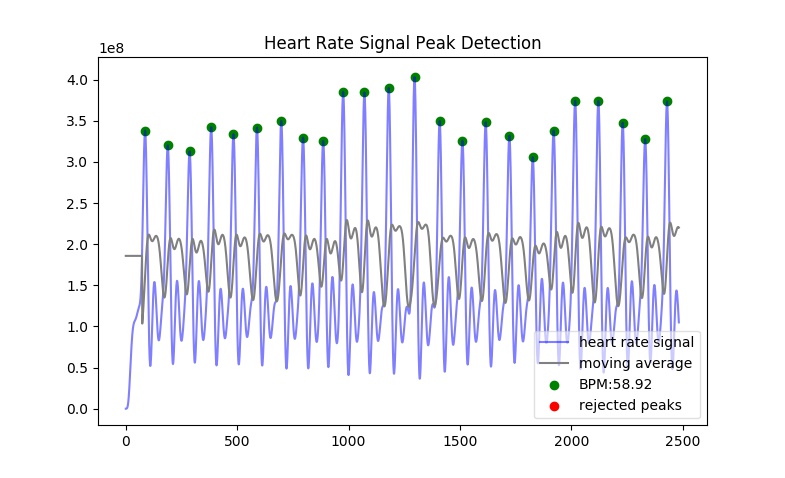
A plotting function is included. It plots the original signal and overlays the detected peaks and the rejected peaks (if any were rejected).
Example with the included data.csv example file (recorded at 100.0Hz):
import heartpy as hp

data = hp.get_data('data.csv')
working_data, measures = hp.process(data, 100.0)
hp.plotter(working_data, measures)
This returns:
plotter(working_data, measures, show = True, title = 'Heart Rate Signal Peak Detection') has two required arguments:
- working_data The working data
dict{}container returned by theprocess()function. - measures The measures
dict{}container returned by theprocess()function.
Several optional arguments are available:
- show _optional_: if set to True a plot is visualised, if set to False a matplotlib.pyplot object is returned. Default show = True;
- title _optional_: Sets the title of the plot. If not specified, default title is used.
Examples:
import heartpy as hp
hrdata = hp.get_data('data2.csv', column_name='hr')
timerdata = hp.get_data('data2.csv', column_name='timer')

working_data, measures = hp.process(hrdata, hp.get_samplerate_mstimer(timerdata))

#plot with different title
hp.plotter(working_data, measures, title='Heart Beat Detection on Noisy Signal')
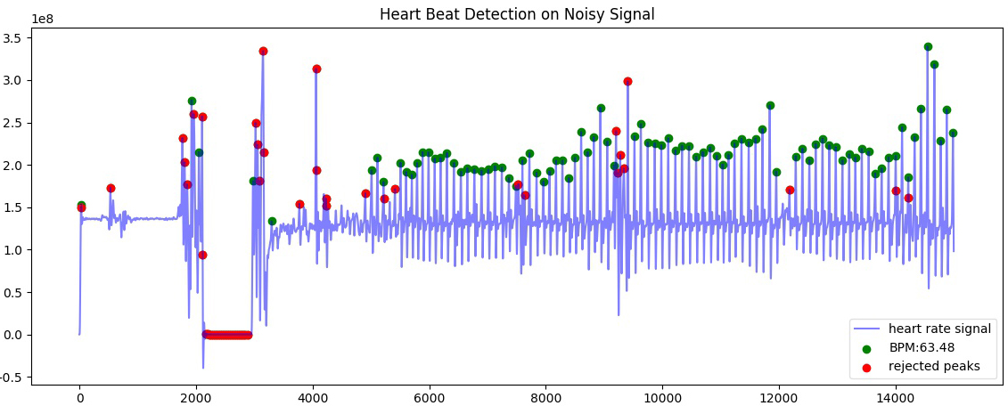
Measures are only calculated for non-rejected peaks and intervals between two non-rejected peaks. Rejected detections do not influence the calculated measures.
By default a plot is visualised when plotter() is called. The function returns a matplotlib.pyplot object if the argument show=False is passed:
working_data, measures = hp.process(hrdata, hp.get_samplerate_mstimer(timerdata))
plot_object = hp.plotter(working_data, measures, show=False)
This returns:
<module 'matplotlib.pyplot' [...]>
Object can then be saved, appended to, or visualised:
working_data, measures = hp.process(hrdata, hp.get_samplerate_mstimer(timerdata))
plot_object = hp.plotter(working_data, measures, show=False)

plot_object.savefig('plot_1.jpg') #saves the plot as JPEG image.

plot_object.show() #displays plot
Plotting results of segmentwise analysis
After calling process_segmentwise(), the returned working_data and measures contain analysis results on the segmented data. This can be visualised using the function segment_plotter():
segment_plotter(working_data, measures, title='Heart Rate Signal Peak Detection', path = '', start=0, end=None, step=1). The function has two required arguments:
- working_data The working data
dict{}container returned by theprocess_segmentwise()function. - measures The measures
dict{}container returned by theprocess_segmentwise()function.
Several optional arguments are available:
- title _optional_: Sets the title of the plot. If not specified, default title is used.
- path _optional_: Where to save the plots. Folder will be created if it doesn’t exist.
- start _optional_: segment index to start at, default = 0, beginning of segments.
- end _optional_: plotting stops when this segment index is reached. Default=None, which is interpreted as meaning plot until end of segment list.
- step _optional_: the stepsize of the plotting. Every step’th segment will be visualised. Default=1, meaning every segment.
Getting heart rate over time
There may be situations where you have a long heart rate signal, and want to compute how the heart rate measures change over time in the signal. HeartPy includes the process_segmentwise function that does just that!
Usage works like this:
working_data, measures = hp.process_segmentwise(data, sample_rate=100.0, segment_width = 40, segment_overlap = 0.25)
What this will do is segment the data into sections of 40 seconds each. In this example each window will have an overlap with the previous window of 25%, meaning each iteration the 40 second window moves by 30 seconds.
process_segmentwist() expects two arguments: - data: 1-d numpy array or list containing heart rate data - sample_rate: the sample rate with which the data is collected, in Hz
Several optional arguments are possible:
- segment_width: the width of the window used, in seconds.
- segment_overlap: the fraction of overlap between adjacent windows: 0 <= segment_overlap < 1.0
- replace_outliers: bool, whether to replace outliers in the computed measures with the median
- segment_min_size: When segmenting, the tail end of the data if often shorter than the specified size in segment_width. The tail end is only included if it is longer than the segment_min_size. Default = 20. Setting this too low is not recommended as it may make peak fitting unstable, and it also doesn’t make much sense from a biosignal analysis perspective to use very short data segments.
- outlier_method: which outlier detection method to use. The interquartile-range (‘iqr’) or modified z-score (‘z-score’) methods are available as of now. Default: ‘iqr’
- mode: ‘fast’ or ‘full’. The ‘fast’ method detects peaks over the entire signal, then segments and computes heart rate and heart rate variability measures. The ‘full’ method segments the data first, then runs the full analysis pipelin on each segment. For small numbers of segments (<10), there is not much difference and the fast method can actually be slower. The more segments there are, the larger the difference becomes. By default you should choose the ‘fast’ method. If there are problems with peak fitting, consider trying the ‘full’ method.
- **kwargs*: you can pass all the arguments normally passed to the process() function at the end of the arguments here as well. These will be passed on and used in the analysis. Example:
working_data, measures = hp.process_segmentwise(data, sample_rate=100.0, segment_width = 40, segment_overlap = 0.25, calc_freq=True, reject_segmentwise=True, report_time=True)
In this example the last three arguments will be passed on the the process() function and used in the analysis. For a full list of arguments that process() supports, see the Basic Example
Example Notebooks are available for further reading!
If you’re looking for a few hands-on examples on how to get started with HeartPy, have a look at the links below! These notebooks show how to handle various analysis tasks with HeartPy, from smartwatch data, smart ring data, regular PPG, and regular (and very noisy) ECG. The notebooks sometimes don’t render through the github engine, so either open them locally, or use an online viewer like [nbviewer](https://nbviewer.jupyter.org/).
We recommend you follow the notebooks in order: - [1. Analysing a PPG signal](https://github.com/paulvangentcom/heartrate_analysis_python/blob/master/examples/1_regular_PPG/Analysing_a_PPG_signal.ipynb), a notebook for starting out with HeartPy using built-in examples. - [2. Analysing an ECG signal](https://github.com/paulvangentcom/heartrate_analysis_python/blob/master/examples/2_regular_ECG/Analysing_a_regular_ECG_signal.ipynb), a notebook for working with HeartPy and typical ECG data. - [3. Analysing smartwatch data](https://github.com/paulvangentcom/heartrate_analysis_python/blob/master/examples/3_smartwatch_data/Analysing_Smartwatch_Data.ipynb), a notebook on analysing low resolution PPG data from a smartwatch. - [4. Analysing smart ring data](https://github.com/paulvangentcom/heartrate_analysis_python/blob/master/examples/4_smartring_data/Analysing_Smart_Ring_Data.ipynb), a notebook on analysing smart ring PPG data. - [5. Analysing noisy ECG data](https://github.com/paulvangentcom/heartrate_analysis_python/blob/master/examples/5_noisy_ECG/Analysing_Noisy_ECG.ipynb), an advanced notebook on working with very noisy ECG data, using data from the MIT-BIH noise stress test dataset.